News & Updates: Data in Practice: PivotTable Basics
Data in Practice: PivotTable Basics
Posted by Marie Jonas
PivotTables are a surprisingly straightforward and highly underutilized Excel tool, that can serve to quickly organize and present critical information in a case. Ask my colleagues: I find uses for PivotTables in nearly every data set I work with.
Let’s start with the data set we worked with for table formatting, some employee time entries, available here.
Inserting a Pivot Table
Click on any cell in the table, press CTRL+A to select just the table (you can manually do the same, but make sure to select only your data set). Then navigate to the “Insert” tab on your top ribbon, and click on the button at the far left, “PivotTable.”
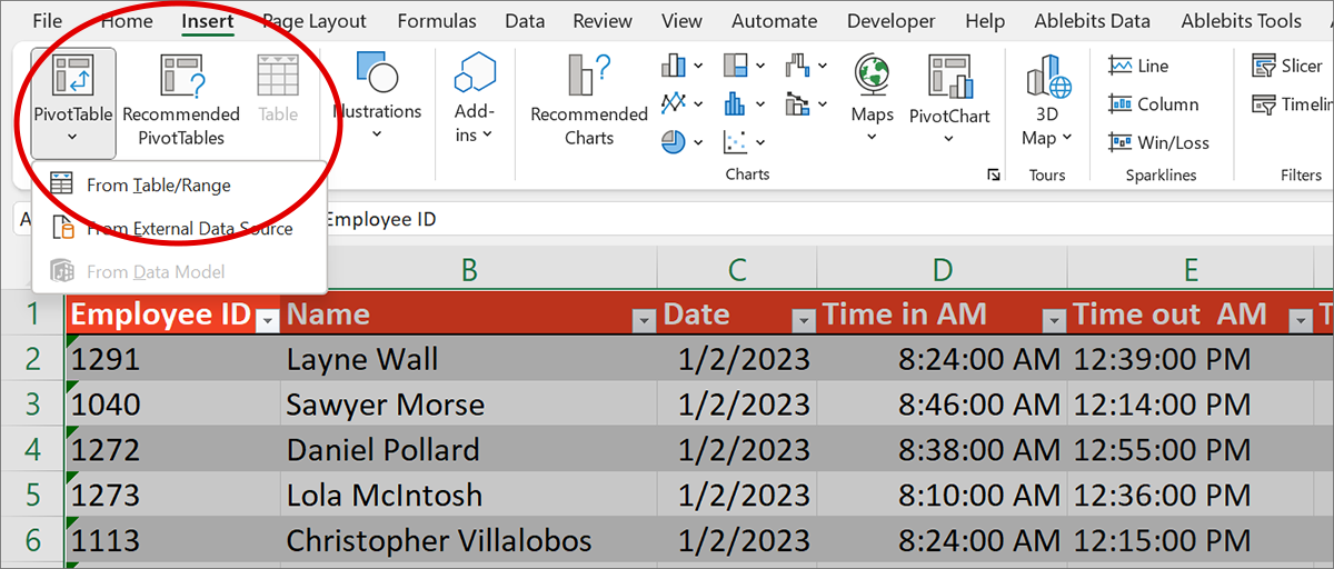
You will get a pop-up like this. Select “New Worksheet” and click OK.
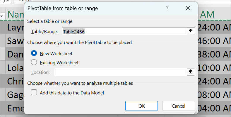
NOTE: What is displayed in the Table/Range field is the name of the table (because this set of data is formatted as a Table in Excel). If your data is not formatted as a table, the range of information you have selected will display with cell references (e.g., A1:H52).
A new sheet will appear in your workbook, and you will automatically be navigated there – staring at mostly a blank screen with the following prompt.
So, what now?
Building Your Table
To start, take a look at the PivotTable fields. They will be visible when you click on a cell in the blank PivotTable box shown above, generally at the right side of your window. Each field listed corresponds to a column of data in the source table. PivotTables provide a way to aggregate and compare fields in your tables with one another.
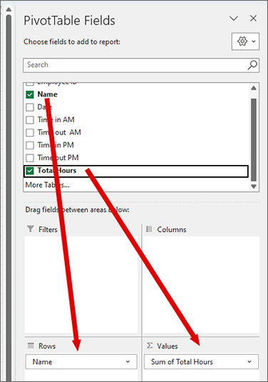
Let’s start with a basic example. Say you want to see the number of hours that each employee worked. The two fields (columns from your data set) that you are working with are Name and Total Hours (note, you must have the hours formatted as numbers, not text, for this summary to work). In this example, I want each employee’s name to be listed on a row, with the total hours they worked as my output.
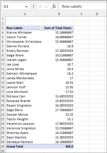
I simply need to drag the respective field to the “Rows” and “Values” menu in the PivotTable fields menu, as shown below. The output in my PivotTable includes the Sum of Total Hours, as shown in the column header.
You instantly can see the total hours worked for all employees on the list.
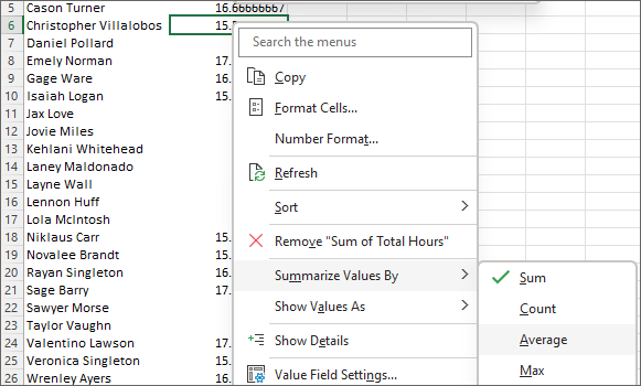
By right-clicking one of the output numbers, you can change the summary data that is displayed.
Say, instead of seeing the total time worked, you wanted to see the average time each employee spent working.
Right click on any number in the Sum of Total Hours column, navigate to “Summarize Values By” and select “Average” rather than “Sum.”
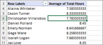
By electing to summarize the values differently, Excel will instantly generate a mean of each instance of that employee’s total hours from our underlying data.
There you have it! The tip of the PivotTable iceberg.
Now let’s take a closer look at what’s being displayed.
Understanding Source Data
To clarify what data is being displayed, let’s take a specific example – Alaina Whitaker. From our PivotTable summary data, we see she worked a total of 15.167 hours, or an average of 7.583 hours per day.
If you navigate back to your underlying data sheet, you can see where exactly those numbers are coming from. Filtering by Alaina’s name gives us the following data.
The values we are looking at are drawn from the “Total Hours” column. We can see that the totals are 7.6333 and 7.5333 respectively. The sum of those two numbers is 15.167. Divided by the two days of data that we have, it generates an average of 7.583.
The practical applications of this tool in legal contexts are incredibly broad, a subject I will dive into more deeply in later posts.
Sheet Cheat
The Sheet Cheat will feature a short excel function or data tool for readers to try out. Please share your favorite cheat via email, and I may include it in a future post!You may have been in this position – you want to reference a specific cell in a spreadsheet, but when you cut and paste the reference into another cell, suddenly the reference moves. Often that’s helpful! Sometimes, it’s not.
Let’s work through this with an example. I have a task list that might look something like this.
NOTE: With rare exception, remember anything preceded by an equal sign in Excel will be read as a “function” (telling Excel to do something).
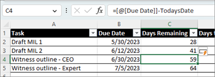
I built a quick function to calculate the difference between the task’s due date and today’s date – but it doesn’t work how I intended. The top row calculates the difference correctly, referencing the cell with Today’s date (G2). But when it filled in the rest, the references changed – to G3, G4, and G5 as the rows ascended. That’s not what I wanted.
When the cell references change like this, as the location of the destination cell for a function changes, it is called a “relative” cell reference.
What we need here is an “absolute” reference – one that doesn’t move when you cut and paste. There are two easy ways to do this:
1. Denote absolute cell references with a dollar sign.
The most common way to mark an absolute cell reference is with a dollar sign. To do this, simply type a dollar sign in front of the column and row, like this:
The dollar in front of the “G” tells the reference to stay in the same column, while the one preceding the number, tells the reference to stay in the same row. Cut and paste, and the cell reference to G2 remains fixed.
2. Denote an absolute cell reference with a cell name.
To do this, click on the cell you want to reference, navigate to the box to the left of the function bar where the cell number is displayed, and 


I named the cell “TodaysDate.” Now I can simply write the cell name in a function when I want to reference it. Populated into my table, it now automatically – and absolutely – references the named cell.
I like this second method because it also serves as a helpful reminder of the data that you are referencing.
Data permeates every aspect of legal practice. Data in Practice is a bimonthly feature to provide practical tools for attorneys to better organize, manipulate, and understand data. Whether it’s working with basic case information, preparing document productions, or conducting exposure analyses, a more robust knowledge of Excel is guaranteed to streamline your work. A few simple tools can help attorneys more efficiently and effectively represent their clients, and better navigate a professional landscape inundated with big data.
Marie Jonas is a Partner in Folger Levin’s litigation practice group. Marie has over a decade of hands-on experience working with Excel in all aspects of her practice: ranging from investigations to trial. If you have an idea for a topic involving practical data tips for lawyers, she can be reached at mjonas@folgerlevin.com.

